NDVI time series

Contents

NDVI time series#

Developed by Lucas Ferreira

# Importing libraries
import rasterio
import xarray
import rioxarray
from pathlib import Path
import matplotlib.pyplot as plt
import pandas as pd

# If you don't have these libraries, you can install them using conda
# conda install -c conda-forge rasterio
# conda install -c conda-forge xarray
# conda install -c conda-forge rioxarray
# conda install -c conda-forge pandas
# conda install matplotlib

---------------------------------------------------------------------------
ModuleNotFoundError                       Traceback (most recent call last)
~\AppData\Local\Temp\ipykernel_22720\1276475333.py in <module>
      1 # Importing libraries
      2 import rasterio
----> 3 import xarray
      4 import rioxarray
      5 from pathlib import Path

ModuleNotFoundError: No module named 'xarray'

NDVI time series#

The dataset is composed of 4 Sentinel-2 images.
Each image is a subset a full Sentinel-2 tile.
Each image has 4 bands: Blue, Green, Red, and NIR.
The date of each image is encoded in the filename.

# Open the dataset
folder = 'dataset/'
# Let's list all the tif files in the folder
geotiff_files = list(Path(folder).glob('*.tif'))
geotiff_files

[WindowsPath('dataset/sample_s2_2022-02-14.tif'),
 WindowsPath('dataset/sample_s2_2022-03-26.tif'),
 WindowsPath('dataset/sample_s2_2022-06-04.tif'),
 WindowsPath('dataset/sample_s2_2022-06-24.tif')]

# Extracting dates embedded in the filenames
dates = [f.name.split('_')[2].split('.')[0] for f in geotiff_files]
# Converting the dates to datetime objects
dates = [pd.to_datetime(d) for d in dates]
dates

[Timestamp('2022-02-14 00:00:00'),
 Timestamp('2022-03-26 00:00:00'),
 Timestamp('2022-06-04 00:00:00'),
 Timestamp('2022-06-24 00:00:00')]

Handling files using rasterio#

Exploring the dataset#

# Open the first file
with rasterio.open(geotiff_files[0]) as src:
    # The parameter masked=True, tells rasterio to return a masked array,
    # where the possible invalid values are masked.
    first_image = src.read(masked=True)

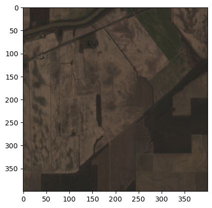
# Lets plot the RGB bands using matplotlib
# Select the RGB bands
rgb_idx = [2, 1, 0]
rgb_image = first_image[rgb_idx, :, :]
# We need to transpose the array to get the correct shape,
# as matplotlib expects the channels to be the last dimension
# and rasterio returns the channels as the first dimension.
rgb_image = rgb_image.transpose(1, 2, 0)
plt.imshow(rgb_image)
plt.show()

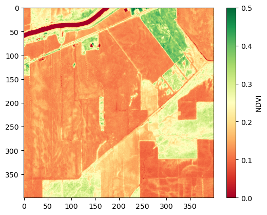
../../_images/96c1d802770ee0e2d87383c28fbbe840e4eb262e31db7235740b7302aa228767.png

# Compute and plot NDVI
def compute_ndvi(image):
    red_idx = [2]
    nir_idx = [3]
    red_band = image[red_idx, :, :]
    nir_band = image[nir_idx, :, :]
    ndvi = (nir_band - red_band) / (nir_band + red_band)
    return ndvi

ndvi = compute_ndvi(first_image)
ndvi = ndvi.transpose(1, 2, 0)
plt.imshow(ndvi, cmap='RdYlGn', vmin=0, vmax=0.5)
plt.colorbar(label='NDVI')
plt.show()

../../_images/6d0f9766e8578aa4c9fafaa0fe97311c8989d7d9b51828e04a79391914cd231f.png

Computing and plotting NDVI across time#

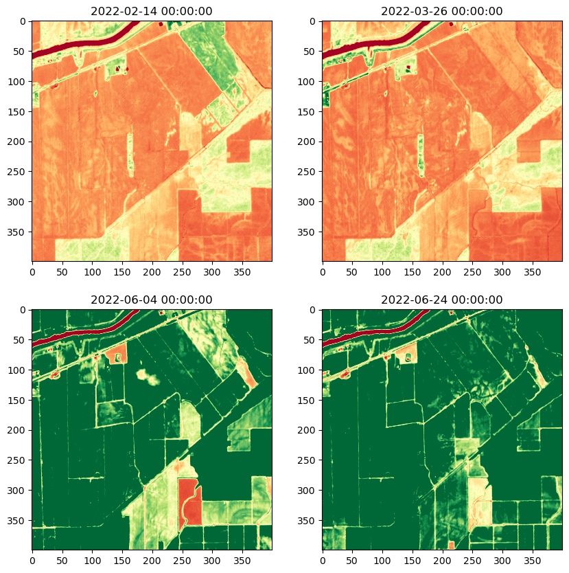
# Read all the images in the folder
images = []
for file in geotiff_files:
    with rasterio.open(file) as src:
        images.append(src.read(masked=True))

# Compute the NDVI for all the images
ndvi_images = []
for image in images:
    ndvi = compute_ndvi(image)
    ndvi_images.append(ndvi)

# Plot all NDVI images
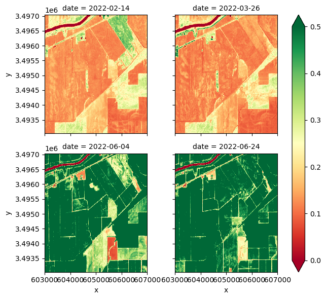
fig = plt.figure(figsize=(10, 10))
for i, ndvi in enumerate(ndvi_images):
    ax = fig.add_subplot(2, 2, i+1)
    ndvi = ndvi.transpose(1, 2, 0)
    date = dates[i]
    ax.set_title(date)
    ax.imshow(ndvi, cmap='RdYlGn', vmin=0, vmax=0.5)
plt.show()

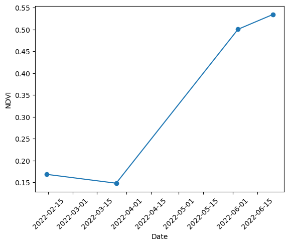
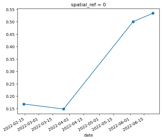
../../_images/ee7bb3e1d07603b8fad497d9b55955954a42130d487576939e189d78f6a76668.png

# Now let's create n NDVI time series. For this we will compute the mean NDVI for each image/date.
mean_ndvi_values = []
for image in ndvi_images:
    mean_ndvi = image.mean()
    mean_ndvi_values.append(mean_ndvi)

# Plot the time series
plt.plot(dates, mean_ndvi_values, 'o-')
plt.ylabel('NDVI')
plt.xlabel('Date')
plt.xticks(rotation=45)
plt.show()

../../_images/655322e55995ce297655e0cedca03a109486eefae98a07aba56ed667e61904db.png

Conclusion#

Both rasterio and xarray are great libraries for working with raster data.
When handling multitemporal data, xarray is probably a better choice.